But what does “using AI tools” actually mean? A developer who accepts tab completions and one who delegates entire features to autonomous agents are both counted in the same adoption statistics. The variation in how developers use these tools is enormous—and mostly invisible in aggregate numbers.
This post uses real survey data to find natural groupings. I clustered 7,041 JetBrains respondents on 75 behavioral features (task frequency, delegation willingness, tool importance, and tool portfolio) and cross-validated against 30,816 Stack Overflow respondents. Then I compared my own Claude Code usage—192 sessions over 15 days—against the clusters that emerged.
The Productivity Paradox
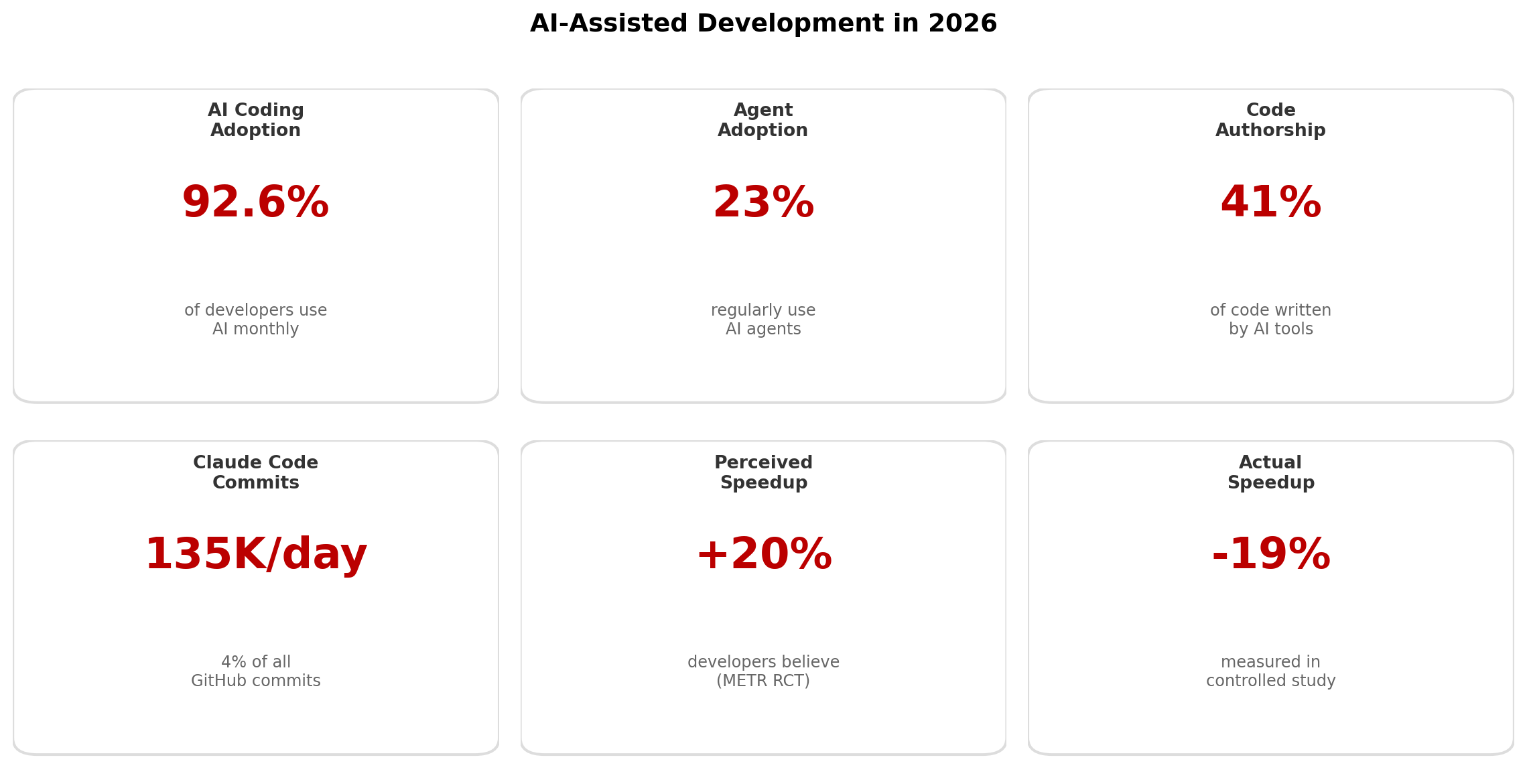
Before the clusters, the headline finding from the research: there is a measurable gap between perceived and actual productivity gains from AI coding tools.
Show code
fig, ax = plt.subplots(figsize=(7.5, 4.5))studies = [ ("Self-reported\n(78% of devs)", 35, "Survey average"), ("METR RCT\n(perceived)", 20, "16 devs believed"), ("METR RCT\n(actual)", -19, "16 devs measured"), ("Faros AI\n(tasks/dev)", 21, "10K+ devs"), ("Faros AI\n(bugs/dev)", 9, "Same cohort"), ("Faros AI\n(review time)", 91, "Bottleneck"), ("Anthropic\n(internal)", 50, "132 engineers"),]labels, values, annotations =zip(*studies)colors = [SCARLET if v >0else DARK_GRAY for v in values]colors[2] = DARK_GRAY # METR actual is negativebars = ax.barh(range(len(labels)), values, color=colors, height=0.6, edgecolor="white")ax.set_yticks(range(len(labels)))ax.set_yticklabels(labels, fontsize=10)ax.set_xlabel("% Change", fontsize=11)ax.axvline(0, color=DARK_GRAY, linewidth=0.8)ax.set_title("AI Coding Productivity: What Developers Report vs. What Studies Measure", fontsize=13, fontweight="bold", pad=12)for i, (bar, ann) inenumerate(zip(bars, annotations)): x = bar.get_width() offset =2if x >=0else-2 ha ="left"if x >=0else"right" ax.text(x + offset, bar.get_y() + bar.get_height()/2, ann, va="center", ha=ha, fontsize=8, color="#666")ax.spines["top"].set_visible(False)ax.spines["right"].set_visible(False)ax.invert_yaxis()plt.tight_layout()plt.show()
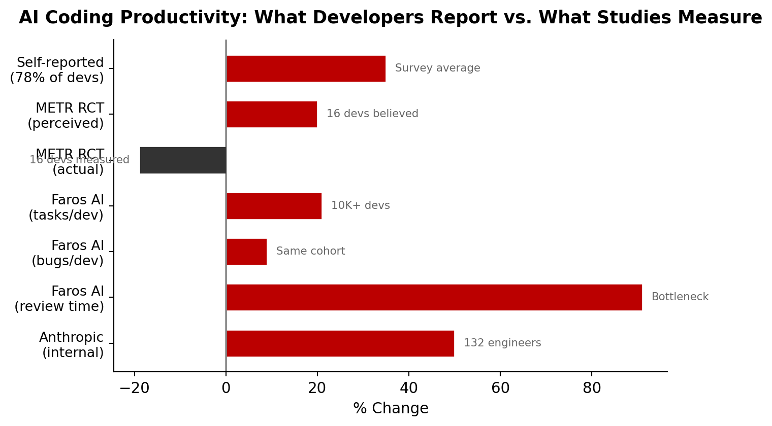
Figure 1: The perception-reality gap in AI coding productivity
The METR randomized controlled trial is particularly striking: experienced open-source developers believed they were 20% faster with AI, but were actually 19% slower. The Faros AI study of 10,000+ developers found individual output increased 21%, but review time ballooned 91% and bugs per developer rose 9%—yielding zero net organizational improvement. The self-reported 35% average gain comes from aggregate survey data across multiple studies; Anthropic’s internal figure of +50% is from their 132-engineer survey of 200K Claude Code transcripts.
This isn’t an argument against AI coding tools. It’s evidence that how you use them matters enormously. The clusters below show just how different those usage patterns are.
Feature engineering (JetBrains): 25 task frequency columns (ordinal 0–5: Never to Every day), 24 delegation willingness columns (ordinal 0–2: Myself/Unsure/Delegate), 16 importance columns (ordinal 0–3), tool count, 6 key tool binary flags, plus agent adoption intent, time saved, and AI sentiment. Total: 75 features.
Dimensionality reduction: StandardScaler → PCA retaining 90% variance → 59 components. t-SNE (perplexity=30) on PCA output for 2D visualization.
Clustering: K-means with k ∈ {3, 4, 5, 6, 7}. Best k selected by silhouette score. DBSCAN as sanity check.
Cross-validation: Same approach on Stack Overflow’s 7 core AI columns (usage frequency, sentiment, accuracy trust, complexity handling, job threat, agent usage, workflow change).
Limitations
JetBrains silhouette = 0.05. The clusters are not well-separated—survey respondents form a continuous distribution, not discrete groups. The clusters are useful as descriptive groupings, not rigid categories.
DBSCAN found 0 natural clusters (all 7,041 points classified as noise), confirming there are no dense, well-separated groups. K-means imposes structure that may not exist.
Stack Overflow’s simpler feature space (7 variables) produces cleaner clusters (silhouette = 0.22) but captures less behavioral nuance.
My personal data is N=1. The session metrics are real but not generalizable.
The JetBrains population skews toward JetBrains IDE users. Stack Overflow skews toward active community members. Neither is representative of all developers.
Show code
fig, (ax1, ax2) = plt.subplots(1, 2, figsize=(10, 4))# JB silhouettejb_k =sorted(meta["k_search_results"].keys(), key=int)jb_sil = [meta["k_search_results"][k]["silhouette"] for k in jb_k]ax1.plot([int(k) for k in jb_k], jb_sil, "o-", color=SCARLET, linewidth=2, markersize=8)ax1.set_xlabel("k (number of clusters)")ax1.set_ylabel("Silhouette Score")ax1.set_title(f"JetBrains (N={meta['n_jb']:,})", fontweight="bold")ax1.axhline(0, color="#ccc", linewidth=0.5)best_jb_k =int(jb_k[np.argmax(jb_sil)])ax1.annotate(f"Best: k={best_jb_k}", (best_jb_k, max(jb_sil)), textcoords="offset points", xytext=(10, 10), fontsize=9, arrowprops=dict(arrowstyle="->", color=SCARLET))ax1.spines["top"].set_visible(False)ax1.spines["right"].set_visible(False)# SO silhouetteso_k =sorted(so["all_results"].keys(), key=int)so_sil = [so["all_results"][k] for k in so_k]ax2.plot([int(k) for k in so_k], so_sil, "o-", color="#336699", linewidth=2, markersize=8)ax2.set_xlabel("k (number of clusters)")ax2.set_ylabel("Silhouette Score")ax2.set_title(f"Stack Overflow (N={so['n_clustered']:,})", fontweight="bold")best_so_k =int(so_k[np.argmax(so_sil)])ax2.annotate(f"Best: k={best_so_k}", (best_so_k, max(so_sil)), textcoords="offset points", xytext=(10, -15), fontsize=9, arrowprops=dict(arrowstyle="->", color="#336699"))ax2.spines["top"].set_visible(False)ax2.spines["right"].set_visible(False)plt.suptitle("Both Surveys Independently Converge on 3 Clusters", fontsize=13, fontweight="bold", y=1.02)plt.tight_layout()plt.show()
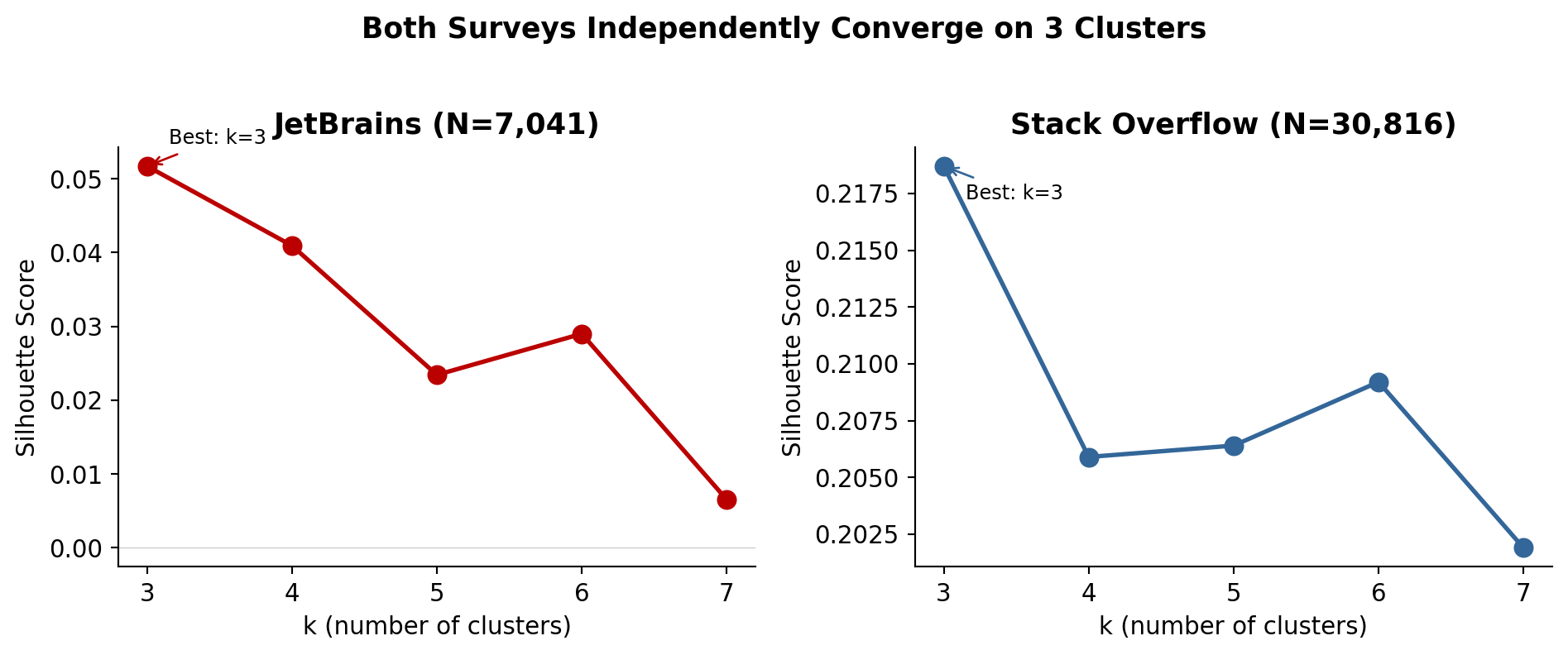
Figure 2: Silhouette scores across k values for both surveys
The Clusters
Three clusters emerged from the JetBrains data. Both surveys independently converged on k=3.
Show code
fig, ax = plt.subplots(figsize=(8, 6))tsne = data["tsne_sample"]for i, cluster inenumerate(clusters): pts = [p for p in tsne if p["cluster"] == cluster["id"]] xs = [p["x"] for p in pts] ys = [p["y"] for p in pts] ax.scatter(xs, ys, s=8, alpha=0.4, c=CLUSTER_COLORS[i], label=f'{cluster["name"]} ({cluster["pct"]}%)')# Robert's positionif"tsne_xy"in robert: ax.scatter(robert["tsne_xy"][0], robert["tsne_xy"][1], s=200, marker="*", c="gold", edgecolors=SCARLET, linewidth=1.5, zorder=10, label="Me (Robert)")ax.set_xlabel("t-SNE 1")ax.set_ylabel("t-SNE 2")ax.set_title("Developer AI Usage Clusters (JetBrains 2025)", fontsize=13, fontweight="bold", pad=12)ax.legend(loc="best", fontsize=9, framealpha=0.9, markerscale=3)ax.spines["top"].set_visible(False)ax.spines["right"].set_visible(False)plt.tight_layout()plt.show()
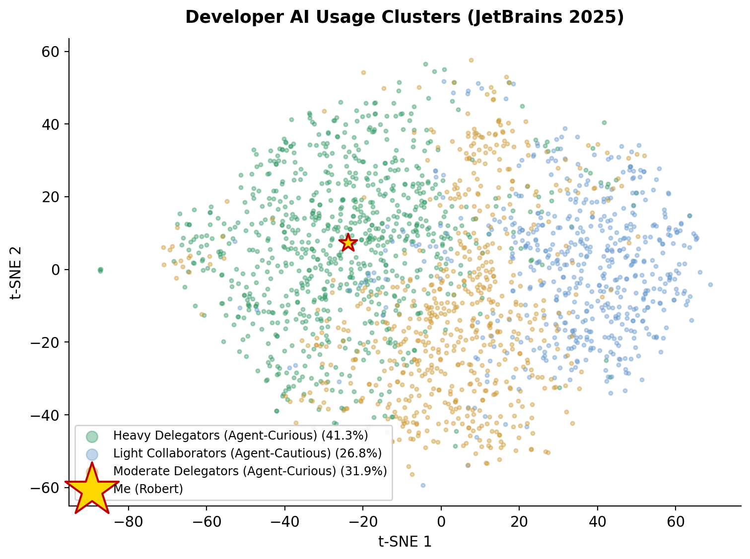
Figure 3: t-SNE projection of 7,041 JetBrains respondents, colored by cluster
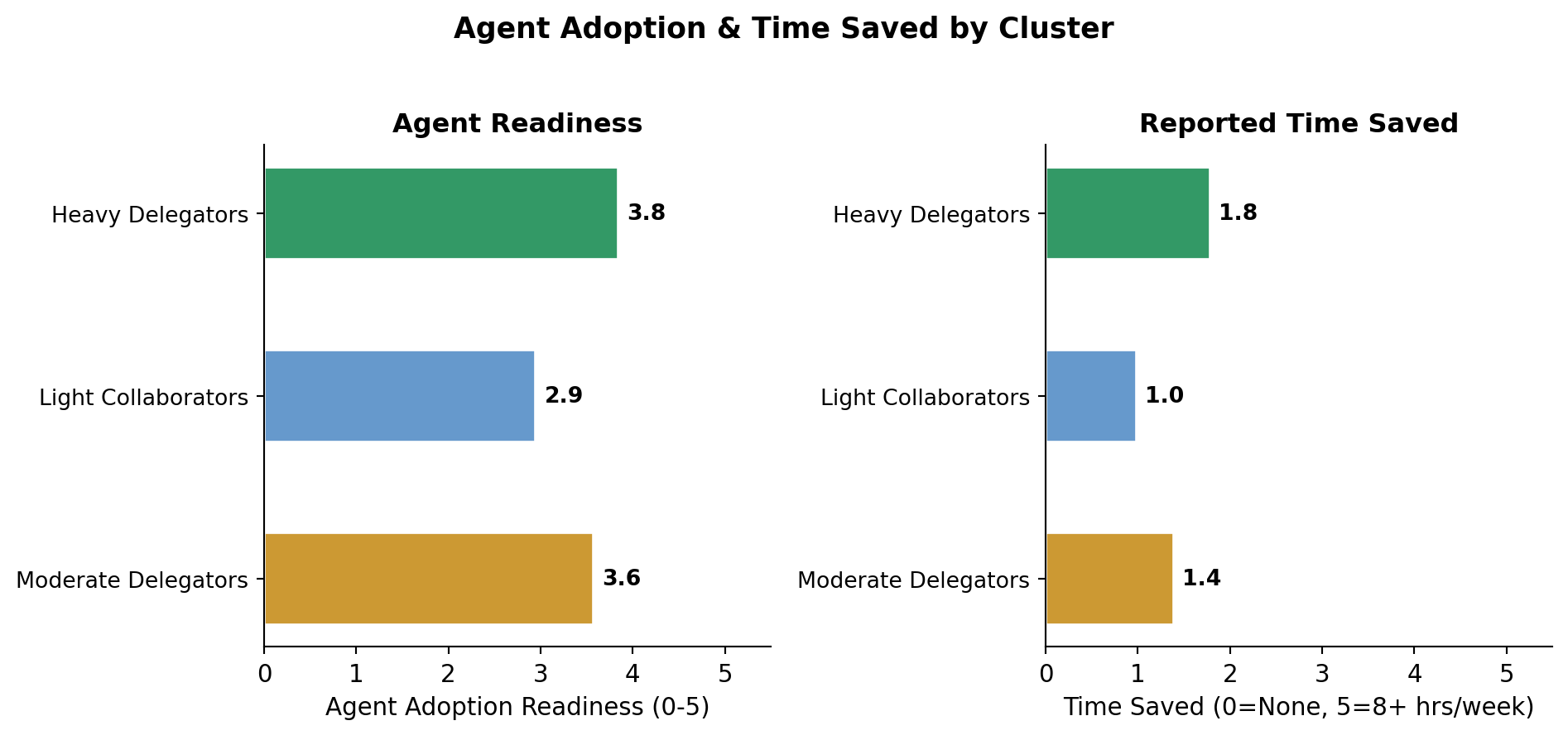
2,910 respondents (41.3%) | Mean tools: 2.4 | Agent readiness: 3.8/5 | Time saved: 1.8/5
Most frequent AI tasks:
Asking questions about software development and coding: ███████████████████░ 4.8/5
Learning new things about coding and software development: ██████████████████░░ 4.7/5
Generating code: ██████████████████░░ 4.6/5
Code completion: ██████████████████░░ 4.6/5
Generating chunks of boilerplate, repetitive code: █████████████████░░░ 4.3/5
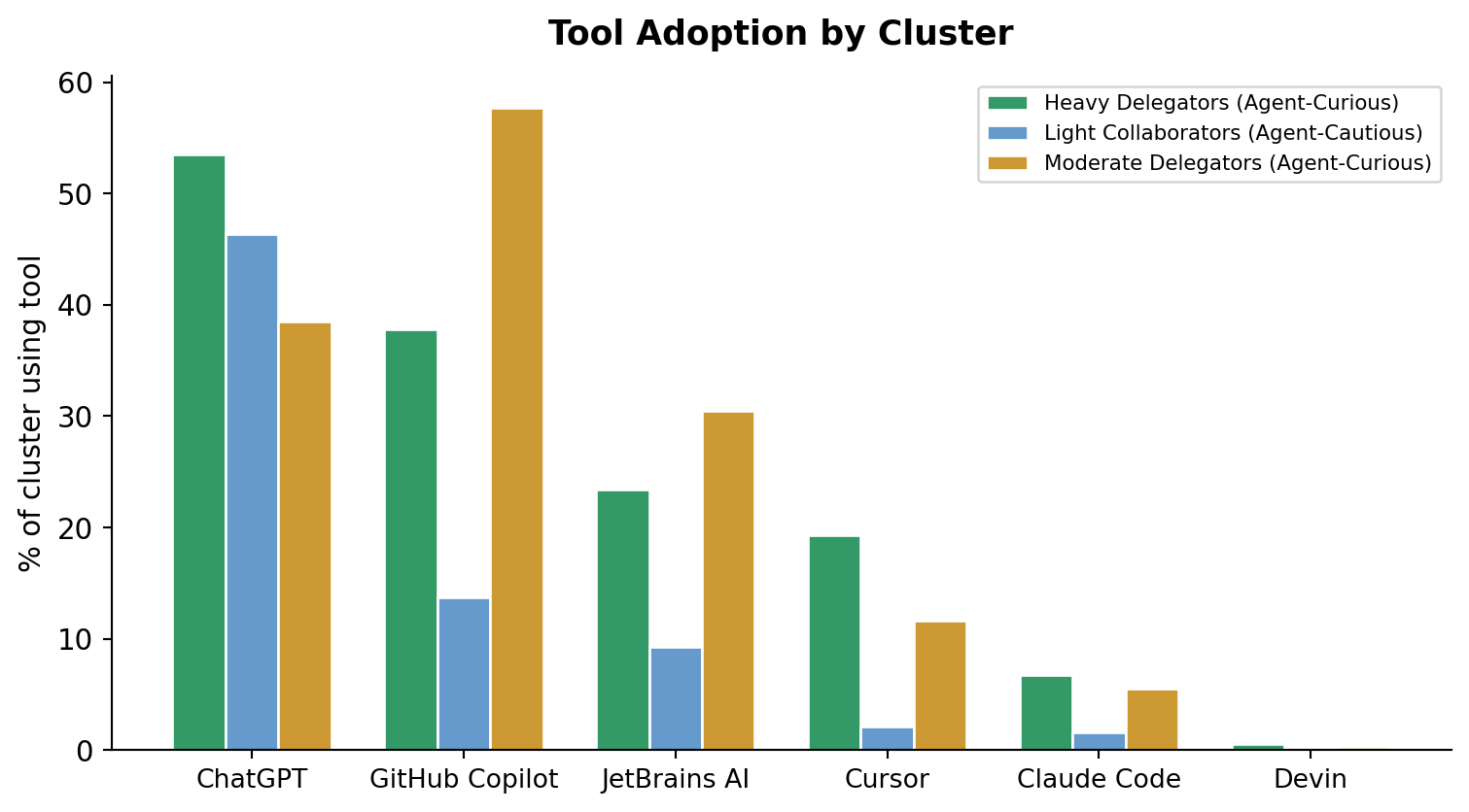
Tool mix: Chatgpt Web / Desktop / Mobile Apps (53.5%), Github Copilot (37.8%), Jetbrains Ai Assistant (23.4%), Cursor (19.3%), Anthropic Claude Code (6.7%)
AI sentiment: Hopeful (32.8%), Excited (29.8%), Anxious (15.0%)
1,884 respondents (26.8%) | Mean tools: 1.2 | Agent readiness: 2.9/5 | Time saved: 1.0/5
Most frequent AI tasks:
Asking questions about software development and coding: ████████████████░░░░ 4.2/5
Learning new things about coding and software development: ███████████████░░░░░ 4.0/5
Brainstorming new ideas: ████████████░░░░░░░░ 3.2/5
Explaining bugs and offering fixes for them: ████████████░░░░░░░░ 3.2/5
Improving or optimizing code: ████████████░░░░░░░░ 3.1/5
Tool mix: Chatgpt Web / Desktop / Mobile Apps (46.4%), Github Copilot (13.7%), Jetbrains Ai Assistant (9.3%), Cursor (2.1%), Anthropic Claude Code (1.6%)
AI sentiment: Uncertain (26.6%), Hopeful (23.9%), Anxious (17.2%)
2,247 respondents (31.9%) | Mean tools: 2.3 | Agent readiness: 3.6/5 | Time saved: 1.4/5
Most frequent AI tasks:
Asking questions about software development and coding: █████████████████░░░ 4.3/5
Code completion: █████████████████░░░ 4.3/5
Learning new things about coding and software development: ████████████████░░░░ 4.1/5
Generating code: ███████████████░░░░░ 3.9/5
Generating code comments or code documentation: ██████████████░░░░░░ 3.6/5
Tool mix: Github Copilot (57.7%), Chatgpt Web / Desktop / Mobile Apps (38.5%), Jetbrains Ai Assistant (30.5%), Cursor (11.6%), Anthropic Claude Code (5.5%)
AI sentiment: Hopeful (24.1%), Uncertain (23.4%), Anxious (21.7%)
Task Frequency Heatmap
Show code
# Select top 15 tasks by variance across clustersall_tasks =list(clusters[0]["task_freq_means"].keys())task_variances = {}for task in all_tasks: vals = [c["task_freq_means"][task] for c in clusters] task_variances[task] = np.var(vals)top_tasks =sorted(task_variances, key=lambda x: -task_variances[x])[:15]# Shorten task namesshort_names = {t: t.replace("Generating ", "Gen. ") .replace("Explaining ", "Explain. ") .replace("Performing ", "Perf. ") .replace("Prompt-based agentic development of features or programs","Agentic development") .replace("Asking questions about software development and coding","Asking dev questions") .replace("Learning new things about coding and software development","Learning new things") .replace("Searching for development-related information on the internet","Searching dev info online") .replace("Search in natural-language queries for code fragments","NL code search") .replace("Suggesting names for classes, functions, variables, etc.","Suggesting names") .replace("Summarizing recent code changes", "Summarizing changes") .replace("chunks of boilerplate, repetitive code", "boilerplate") .replace("code comments or code documentation", "code docs") .replace("Editing code across multiple files", "Multi-file editing") .replace("Improving or optimizing code", "Improving/optimizing") .replace("Converting code to other languages", "Converting languages") .replace("Gen. CLI commands by natural-language description", "Gen. CLI commands") .replace("Gen. internal documentation", "Gen. internal docs") .replace("Gen. user documentation (e.g. manuals, tutorials, release notes)","Gen. user docs") .replace("Gen. commit messages", "Gen. commits") .replace("Refactoring code", "Refactoring") .replace("Debugging code", "Debugging") .replace("Checking code for potential issues", "Code checking")for t in top_tasks}fig, ax = plt.subplots(figsize=(10, 6))heat_data = np.array([[c["task_freq_means"][t] for t in top_tasks] for c in clusters])im = ax.imshow(heat_data, cmap="YlOrRd", aspect="auto", vmin=0, vmax=5)ax.set_xticks(range(len(top_tasks)))ax.set_xticklabels([short_names[t] for t in top_tasks], rotation=45, ha="right", fontsize=9)ax.set_yticks(range(len(clusters)))ax.set_yticklabels([c["name"] for c in clusters], fontsize=10)# Annotate cellsfor i inrange(len(clusters)):for j inrange(len(top_tasks)): val = heat_data[i, j] color ="white"if val >3else DARK_GRAY ax.text(j, i, f"{val:.1f}", ha="center", va="center", fontsize=8, color=color)plt.colorbar(im, ax=ax, label="Frequency (0=Never, 5=Every day)", shrink=0.8)ax.set_title("AI Task Frequency by Cluster (top 15 most-variable tasks)", fontsize=13, fontweight="bold", pad=12)plt.tight_layout()plt.show()
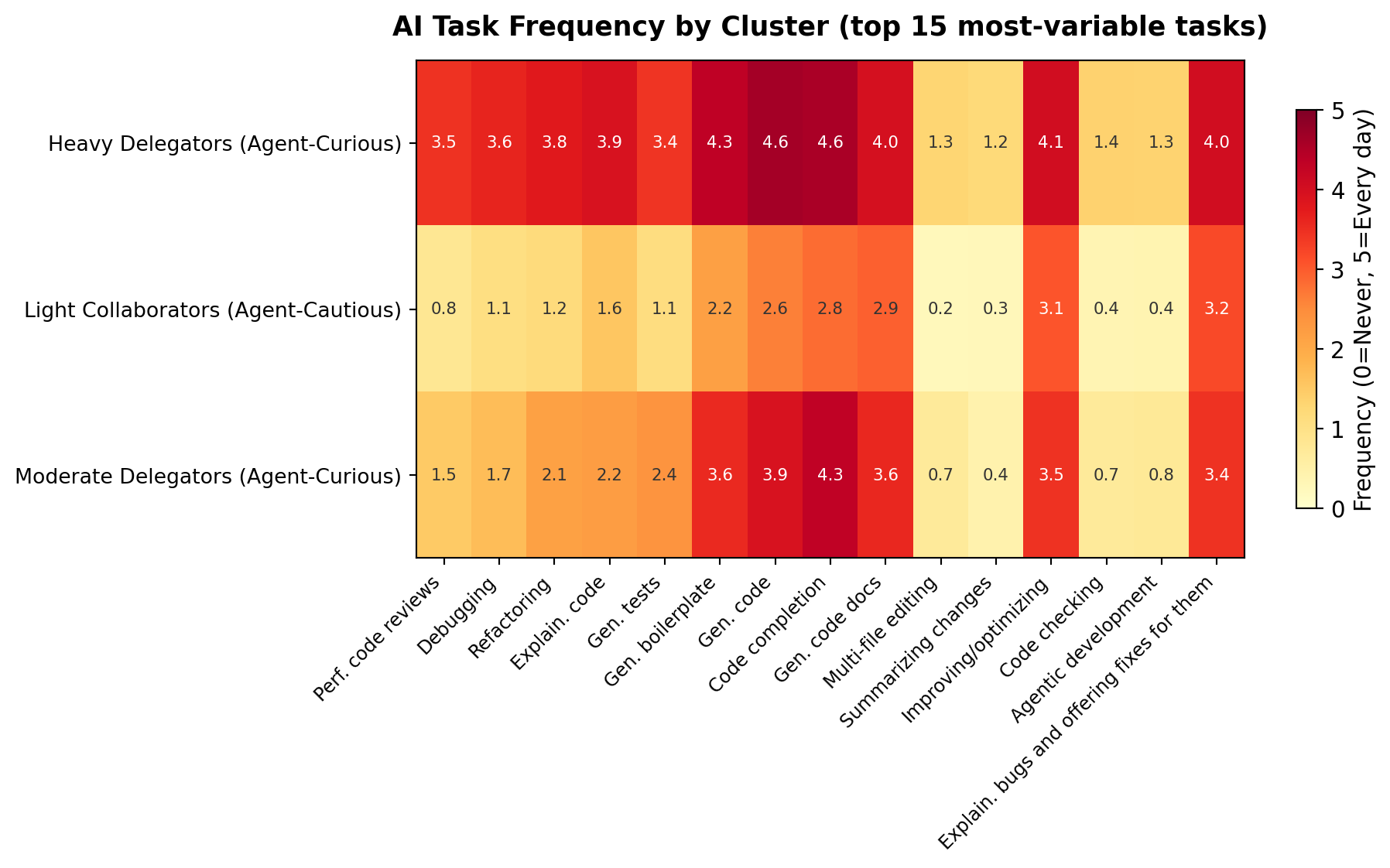
Figure 4: Mean AI task frequency by cluster (0=Never, 5=Every day)
Tool Composition
Show code
fig, ax = plt.subplots(figsize=(8, 4.5))tool_names_map = {"chatgpt_web_/_desktop_/_mobile_apps": "ChatGPT","github_copilot": "GitHub Copilot","jetbrains_ai_assistant": "JetBrains AI","cursor": "Cursor","anthropic_claude_code": "Claude Code","devin": "Devin",}tool_keys =list(tool_names_map.keys())x = np.arange(len(tool_keys))width =0.25for i, c inenumerate(clusters): vals = [c["tool_pcts"].get(t, 0) for t in tool_keys] offset = (i -len(clusters) /2+0.5) * width bars = ax.bar(x + offset, vals, width, label=c["name"], color=CLUSTER_COLORS[i], edgecolor="white")ax.set_xticks(x)ax.set_xticklabels([tool_names_map[t] for t in tool_keys], fontsize=10)ax.set_ylabel("% of cluster using tool")ax.set_title("Tool Adoption by Cluster", fontsize=13, fontweight="bold", pad=12)ax.legend(fontsize=8, loc="upper right")ax.spines["top"].set_visible(False)ax.spines["right"].set_visible(False)plt.tight_layout()plt.show()
Figure 5: Tool adoption rates by cluster
Delegation Willingness
Show code
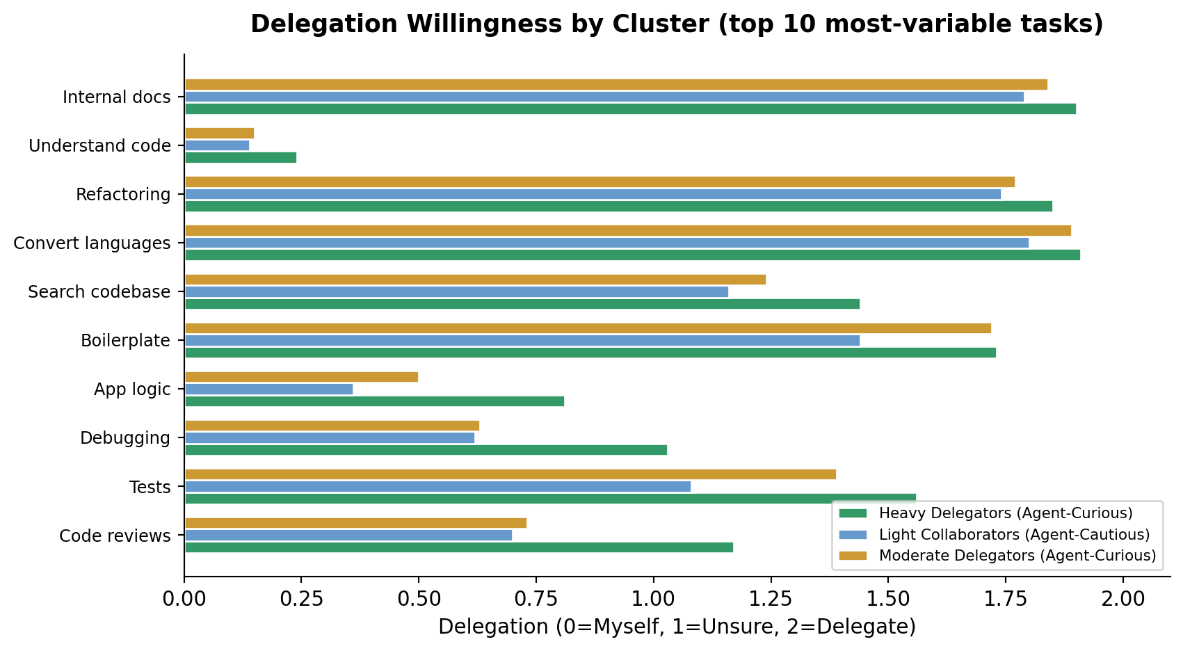
# Top 10 most variable delegation tasksdel_tasks =list(clusters[0]["delegation_means"].keys())del_vars = {}for task in del_tasks: vals = [c["delegation_means"][task] for c in clusters] del_vars[task] = np.var(vals)top_del =sorted(del_vars, key=lambda x: -del_vars[x])[:10]fig, ax = plt.subplots(figsize=(9, 5))short_del = { t: t.replace("Writing ", "") .replace("Performing ", "") .replace("Searching for development-related information on the internet","Search dev info online") .replace("Searching for code fragments inside the codebase", "Search codebase") .replace("Understanding recent code changes", "Understand changes") .replace("Understanding code", "Understand code") .replace("Explaining bugs and offering fixes for them", "Explain/fix bugs") .replace("Checking code for potential issues", "Check code issues") .replace("Improving or optimizing code", "Improve/optimize") .replace("Creating project-related content, such as tasks, comments, descriptions, etc.","Project content") .replace("Converting code to other languages", "Convert languages") .replace("Communicating through email and messaging", "Email/messaging") .replace("actions in the terminal / CLI", "Terminal/CLI") .replace("code reviews", "Code reviews") .replace("Brainstorming new ideas", "Brainstorming") .replace("Summarizing recent code changes", "Summarize changes") .replace("reports or whitepapers", "Reports") .replace("application logic code", "App logic") .replace("boilerplate, repetitive code", "Boilerplate") .replace("code comments or code documentation", "Code docs") .replace("internal documentation", "Internal docs") .replace("user documentation (e.g. manuals, tutorials, release notes)", "User docs") .replace("commit messages", "Commits") .replace("tests", "Tests")for t in top_del}y = np.arange(len(top_del))height =0.25for i, c inenumerate(clusters): vals = [c["delegation_means"][t] for t in top_del] offset = (i -len(clusters) /2+0.5) * height ax.barh(y + offset, vals, height, label=c["name"], color=CLUSTER_COLORS[i], edgecolor="white")ax.set_yticks(y)ax.set_yticklabels([short_del[t] for t in top_del], fontsize=9)ax.set_xlabel("Delegation (0=Myself, 1=Unsure, 2=Delegate)")ax.set_title("Delegation Willingness by Cluster (top 10 most-variable tasks)", fontsize=13, fontweight="bold", pad=12)ax.legend(fontsize=8, loc="lower right")ax.spines["top"].set_visible(False)ax.spines["right"].set_visible(False)ax.set_xlim(0, 2.1)plt.tight_layout()plt.show()
Figure 6: Mean delegation willingness by cluster (0=Do it myself, 2=Delegate to AI)
Agent Adoption & Time Saved
Show code
fig, (ax1, ax2) = plt.subplots(1, 2, figsize=(10, 4.5))# Agent adoptionnames = [c["name"].split("(")[0].strip() for c in clusters]agent_vals = [c["mean_agent_try"] for c in clusters]bars1 = ax1.barh(range(len(clusters)), agent_vals, color=[CLUSTER_COLORS[i] for i inrange(len(clusters))], height=0.5, edgecolor="white")ax1.set_yticks(range(len(clusters)))ax1.set_yticklabels(names, fontsize=10)ax1.set_xlabel("Agent Adoption Readiness (0-5)")ax1.set_title("Agent Readiness", fontweight="bold", fontsize=12)ax1.set_xlim(0, 5.5)for i, (bar, val) inenumerate(zip(bars1, agent_vals)): ax1.text(bar.get_width() +0.1, bar.get_y() + bar.get_height()/2,f"{val:.1f}", va="center", fontsize=10, fontweight="bold")ax1.spines["top"].set_visible(False)ax1.spines["right"].set_visible(False)ax1.invert_yaxis()# Time savedtime_vals = [c["mean_time_saving"] for c in clusters]bars2 = ax2.barh(range(len(clusters)), time_vals, color=[CLUSTER_COLORS[i] for i inrange(len(clusters))], height=0.5, edgecolor="white")ax2.set_yticks(range(len(clusters)))ax2.set_yticklabels(names, fontsize=10)ax2.set_xlabel("Time Saved (0=None, 5=8+ hrs/week)")ax2.set_title("Reported Time Saved", fontweight="bold", fontsize=12)ax2.set_xlim(0, 5.5)for i, (bar, val) inenumerate(zip(bars2, time_vals)): ax2.text(bar.get_width() +0.1, bar.get_y() + bar.get_height()/2,f"{val:.1f}", va="center", fontsize=10, fontweight="bold")ax2.spines["top"].set_visible(False)ax2.spines["right"].set_visible(False)ax2.invert_yaxis()plt.suptitle("Agent Adoption & Time Saved by Cluster", fontsize=13, fontweight="bold", y=1.02)plt.tight_layout()plt.show()
Figure 7: Agent adoption readiness and time saved per cluster
Claude Code Users
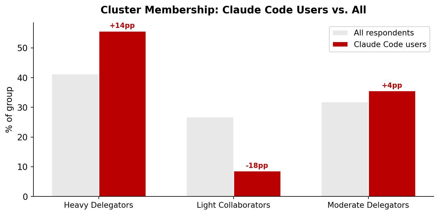
Of the 7,041 respondents, 348 use Claude Code. They cluster very differently from the general population.
Show code
fig, ax = plt.subplots(figsize=(8, 4))cluster_names = [c["name"].split("(")[0].strip() for c in clusters]cc_dist = cc["cluster_distribution"]all_pcts = [cc_dist[str(c["id"])]["all_pct"] for c in clusters]cc_pcts = [cc_dist[str(c["id"])]["cc_pct"] for c in clusters]x = np.arange(len(clusters))width =0.35ax.bar(x - width/2, all_pcts, width, label="All respondents", color=LIGHT_GRAY, edgecolor="white")ax.bar(x + width/2, cc_pcts, width, label="Claude Code users", color=SCARLET, edgecolor="white")ax.set_xticks(x)ax.set_xticklabels(cluster_names, fontsize=10)ax.set_ylabel("% of group")ax.set_title("Cluster Membership: Claude Code Users vs. All", fontsize=13, fontweight="bold", pad=12)ax.legend(fontsize=10)ax.spines["top"].set_visible(False)ax.spines["right"].set_visible(False)# Annotate the differencefor i inrange(len(clusters)): diff = cc_pcts[i] - all_pcts[i]ifabs(diff) >3: sign ="+"if diff >0else"" ax.text(x[i] + width/2, cc_pcts[i] +1, f"{sign}{diff:.0f}pp", ha="center", fontsize=9, fontweight="bold", color=SCARLET)plt.tight_layout()plt.show()
Figure 8: Claude Code users concentrate in the most active cluster
The difference is statistically significant (chi2=65.01, p<0.001, df=2).
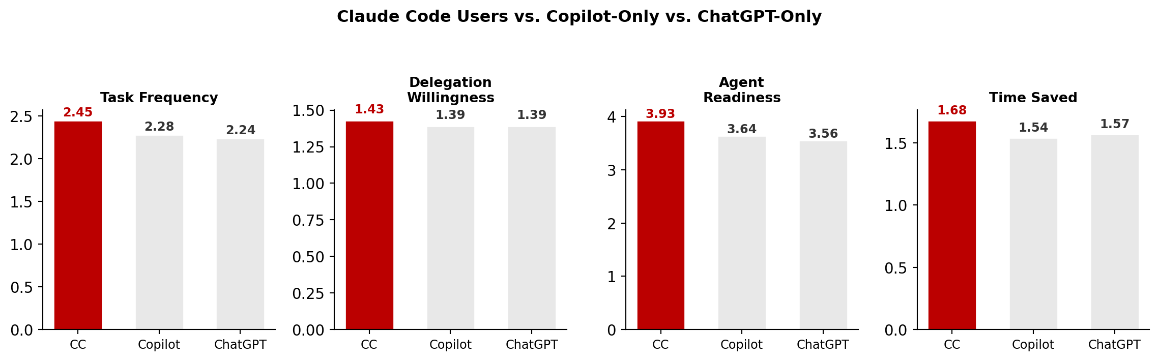
Claude Code vs. Copilot vs. ChatGPT
Show code
comps = cc["tool_comparisons"]tools = ["claude_code", "copilot", "chatgpt"]tool_labels = ["Claude Code\n(N={})".format(comps["claude_code"]["n"]),"Copilot-only\n(N={})".format(comps.get("copilot", {}).get("n", 0)),"ChatGPT-only\n(N={})".format(comps.get("chatgpt", {}).get("n", 0))]metrics = ["mean_task_freq", "mean_delegation", "mean_agent_try", "mean_time_saving"]metric_labels = ["Task Frequency", "Delegation\nWillingness", "Agent\nReadiness", "Time Saved"]fig, axes = plt.subplots(1, 4, figsize=(12, 3.5))for ax, metric, label inzip(axes, metrics, metric_labels): vals = []for t in tools:if t in comps and metric in comps[t]: vals.append(comps[t][metric])else: vals.append(0) colors = [SCARLET, LIGHT_GRAY, LIGHT_GRAY] ax.bar(range(len(tools)), vals, color=colors, edgecolor="white", width=0.6) ax.set_xticks(range(len(tools))) ax.set_xticklabels(["CC", "Copilot", "ChatGPT"], fontsize=9) ax.set_title(label, fontweight="bold", fontsize=10)for j, v inenumerate(vals): ax.text(j, v +0.05, f"{v:.2f}", ha="center", fontsize=9, fontweight="bold", color=SCARLET if j ==0else DARK_GRAY) ax.spines["top"].set_visible(False) ax.spines["right"].set_visible(False)plt.suptitle("Claude Code Users vs. Copilot-Only vs. ChatGPT-Only", fontsize=12, fontweight="bold", y=1.05)plt.tight_layout()plt.show()
Figure 9: Claude Code users show higher task frequency, delegation, and agent readiness
Cross-Validation: Stack Overflow
The Stack Overflow survey asks different questions (sentiment, trust, complexity assessment) but independently produces the same structure: 3 clusters.
From 30,816 respondents with complete data (silhouette = 0.219):
Cluster
Size
AI Usage
Sentiment
Agent Usage
Trust
AI Enthusiasts
11,376 (36.9%)
daily
Very favorable
daily
Somewhat trust
AI Skeptics
7,934 (25.7%)
No, and I don’t plan to
Very unfavorable
No, and I don’t plan to
Highly distrust
AI Enthusiasts
11,506 (37.3%)
daily
Favorable
No, and I don’t plan to
Somewhat distrust
The pattern across both surveys: a large group of active, enthusiastic adopters (~37–41%), a similar-sized group of moderate or cautious users (~32–37%), and a smaller group of skeptics or non-adopters (~26–29%). The same tripartite structure appears despite completely different question sets and populations.
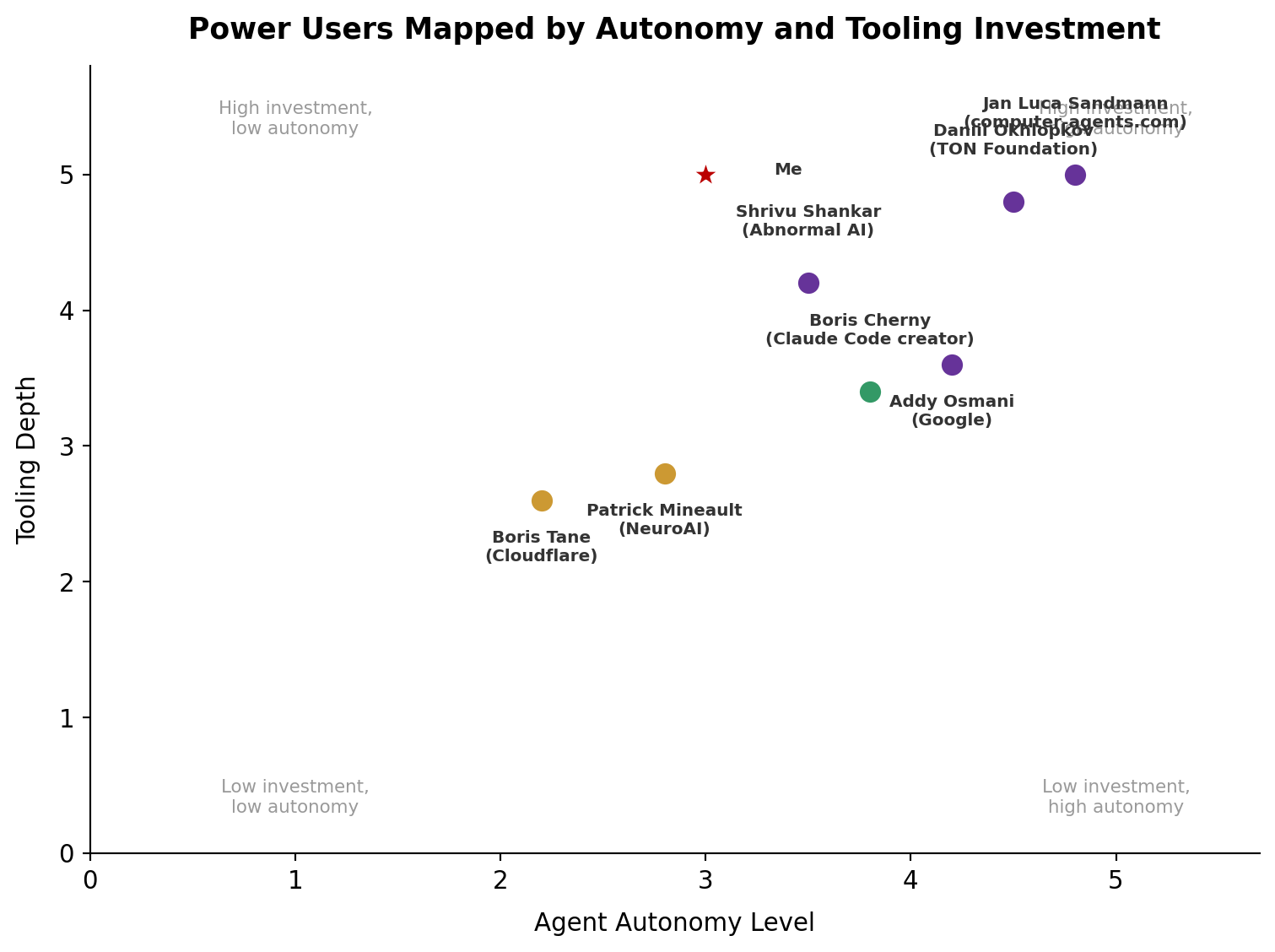
Power Users in the Wild
The clusters above describe the population. But the most informative data points come from named practitioners who have documented their workflows in detail. Here’s how real power users map onto the spectrum.
Figure 10: Named power users mapped onto the archetype spectrum
Boris Cherny (Claude Code’s creator) runs 5 local terminal sessions + 5–10 web sessions simultaneously, ships 20–30 PRs daily, and hasn’t manually edited code since November 2025. His setup is “surprisingly vanilla”—the key is plan mode first, then auto-accept, with verification loops that improve output 2–3x. In cluster terms, he would land squarely in the Heavy Delegators group, with the highest task frequency and delegation scores.
Boris Tane (Engineering Lead, Cloudflare) uses no hooks, skills, or MCP servers—pure workflow discipline. His Research-Plan-Annotate-Implement cycle involves 1–6 annotation rounds where he cherry-picks proposals before Claude writes a line of code. He represents the Moderate Delegators—high engagement but with deliberate human gatekeeping.
Shrivu Shankar (Abnormal AI) maintains a 13KB CLAUDE.md for their monorepo, uses block-at-submit hooks that force agents into test-fix loops before committing, and is migrating away from MCP servers toward CLI wrappers. His team consumes “several billion tokens monthly.”
Addy Osmani (Google) runs adversarial agent teams—competing hypothesis debuggers, parallel security/performance/test reviewers—treating agents like a distributed engineering team with shared task lists and inbox-based messaging.
Patrick Mineault (NeuroAI researcher) runs 5–10 parallel Claude windows, emphasizes “lots of plots” for cheap validation, and warns that AI tools “can produce wrong results faster than ever before”—making metacognition the critical skill for researchers.
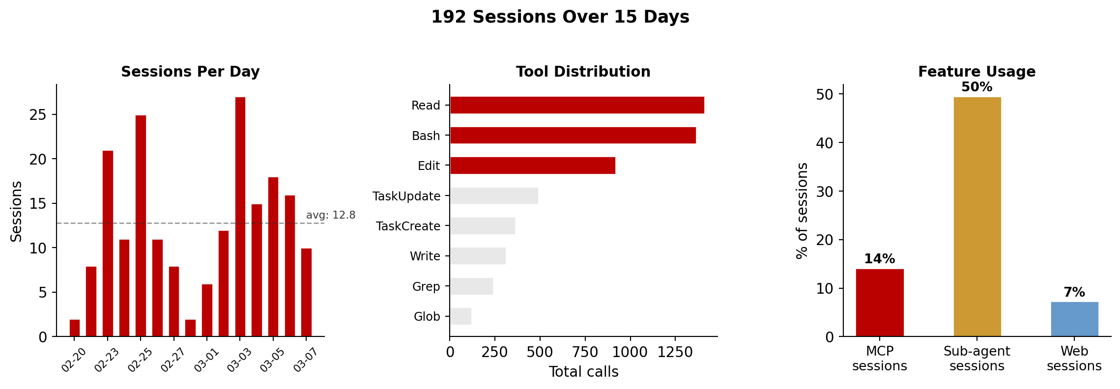
Where I Land
Over 15 days in February–March 2026, I ran 192 sessions totaling 74 hours with Claude Code. The data comes from Claude Code’s session-meta JSON files, which log every tool call, token count, and timestamp.
Show code
fig, axes = plt.subplots(1, 3, figsize=(12, 4))# Daily sessionsif robert.get("daily_sessions"): daily = robert["daily_sessions"] dates =list(daily.keys()) counts =list(daily.values()) short_dates = [d[5:] for d in dates] # MM-DD ax = axes[0] ax.bar(range(len(dates)), counts, color=SCARLET, edgecolor="white", width=0.7) ax.set_xticks(range(0, len(dates), 2)) ax.set_xticklabels([short_dates[i] for i inrange(0, len(dates), 2)], rotation=45, fontsize=8) ax.set_ylabel("Sessions") ax.set_title("Sessions Per Day", fontweight="bold", fontsize=11) ax.axhline(robert["sessions_per_day"], color=DARK_GRAY, linewidth=1, linestyle="--", alpha=0.5) ax.text(len(dates) -1, robert["sessions_per_day"] +0.5,f'avg: {robert["sessions_per_day"]}', fontsize=8, color=DARK_GRAY) ax.spines["top"].set_visible(False) ax.spines["right"].set_visible(False)# Tool distribution (top 8)ax = axes[1]if robert.get("tool_distribution"): tools =list(robert["tool_distribution"].items())[:8] tool_names = [name.replace("mcp__playwright__browser_", "pw:") for name, _ in tools] tool_counts = [count for _, count in tools] colors_bar = [SCARLET if i <3else LIGHT_GRAY for i inrange(len(tools))] ax.barh(range(len(tools)), tool_counts, color=colors_bar, height=0.6, edgecolor="white") ax.set_yticks(range(len(tools))) ax.set_yticklabels(tool_names, fontsize=9) ax.set_xlabel("Total calls") ax.set_title("Tool Distribution", fontweight="bold", fontsize=11) ax.invert_yaxis() ax.spines["top"].set_visible(False) ax.spines["right"].set_visible(False)# Feature flagsax = axes[2]flag_data = [ ("MCP\nsessions", robert.get("pct_mcp_sessions", 0)), ("Sub-agent\nsessions", robert.get("pct_task_sessions", 0)), ("Web\nsessions", robert.get("pct_web_sessions", 0)),]flag_names, flag_vals =zip(*flag_data)ax.bar(range(len(flag_data)), flag_vals, color=[SCARLET, "#cc9933", "#6699cc"], edgecolor="white", width=0.5)ax.set_xticks(range(len(flag_data)))ax.set_xticklabels(flag_names, fontsize=10)ax.set_ylabel("% of sessions")ax.set_title("Feature Usage", fontweight="bold", fontsize=11)for i, v inenumerate(flag_vals): ax.text(i, v +1, f"{v:.0f}%", ha="center", fontsize=10, fontweight="bold")ax.spines["top"].set_visible(False)ax.spines["right"].set_visible(False)plt.suptitle(f"192 Sessions Over 15 Days", fontsize=13, fontweight="bold", y=1.02)plt.tight_layout()plt.show()
Figure 11: My Claude Code usage over 15 days
192
Sessions
12.8
Sessions/day
74.3h
Total time
23.2m
Avg duration
$1,046
Total cost
$70/day
Daily cost
23
Git commits
44,263
Lines added
My projected cluster is Cluster 0 (Heavy Delegators (Agent-Curious))—the most active group. But the numbers reveal trade-offs:
Intensity: 12.8 sessions/day, where the Max plan targets 4–5 hours of complex work daily.
Infrastructure: 6 MCP servers, 7 hooks, 15+ skills, 3 knowledge layers. This is not “just using Claude Code”—it’s building a platform on top of it.
What the numbers don’t show: Diminishing returns are real. Not every session was productive. The sub-agent sessions (42% of all sessions) often burned tokens on exploratory work that led nowhere. The hooks and skills took days to build and still require maintenance.
The honest assessment: I’m an outlier, and not all of that outlier status is productive. The infrastructure investment compounds across sessions, but only if the underlying projects benefit from cross-session memory and automated validation. For a single-project developer, most of this tooling would be overhead.
What Separates Effective Users
Across both the survey data and the practitioner reports, three patterns consistently separate developers who get compounding value from AI tools:
1. Verification as a first-class concern. The cluster with the highest task frequency (Heavy Delegators) also reports the most time saved—but only because they’ve built feedback loops. Boris Cherny calls verification loops the single most important practice: “Give Claude a way to verify its work… this can improve the quality of the final result by a factor of 2–3x.” Simon Willison’s Agentic Engineering Patterns makes the same point through TDD.
2. Persistent context across sessions. The biggest waste in AI coding is re-explaining project conventions every session. CLAUDE.md files, custom rules, knowledge graphs, and memory systems all address this. The JetBrains data shows that multi-tool users (cluster 0, avg 2.4 tools) report nearly twice the time savings of single-tool users (cluster 1, avg 1.2 tools). More tools means more persistent context, not just more features.
3. Separation of planning and implementation. Sessions that blend research, planning, and coding in a single context window tend to exhaust context before finishing. The most effective pattern: plan in session 1 (write a markdown artifact), review it yourself, implement in session 2 with the plan as input. Boris Tane’s 1–6 annotation cycles are an extreme version of this.
We’re in the early innings. Only 23% of developers use AI agents regularly, yet agents already author 4% of all GitHub commits. The gap between adoption of passive AI (autocomplete) and active AI (agents) will close rapidly as tools improve and verification patterns mature.
The question isn’t whether to use agentic coding tools. It’s whether you’re investing in the practices—especially verification—that separate compounding productivity from expensive churn.
Sources
Surveys and Studies
METR RCT Study — 16 experienced developers, 246 tasks, randomized controlled trial